GPS Navigation

Introduction

Navigation with the assistance of a GPS was utilized for the orienteering course at the Priory in Eau Claire. Being able to navigate with a GPS is vital to many because not everyone has access to a compass but almost everyone has a GPS in the form of a smartphone. For this exercise the Juno GPS from trimble was used but we could have used a map on a cell phone if needed.

Methods

Before the navigation occurred the first step was to develop a map and a plan for the course. Instead of doing just 5 points like in a previous exercise we were tasked with doing the entire course. The map was similar to what was made for the previous exercise but with all of the flags marked and a path for us to follow was included. The map was then exported to the Juno to be used in the ArcPad application. While doing the course with the GPS we were also supposed to take points at each flag to ensure that we made it to each since this was also a race.

Figure 1. The map used for the navigation. The black line represents the path followed, black dots are the flags, red triangles are the locations recorded of the flags by the GPS, and the green dot is the starting point of the course. Red areas are no firing zones.

Discussion

Using paintball guns during the exercise definitely got the heart rates going but after finding the first couple of flags we didn’t run into any other teams. Navigating by using the GPS was extremely easy. Issues ran into while using the GPS were minor but it did turn off while halfway through the course and reconnecting to the satellites took what seemed like several minutes. This is mostly due to the amount of tree cover we were under but once it reconnected it worked just fine for the rest of the course.

Conclusion

Using a GPS for not only collecting data but for navigating is an invaluable skill. Even though we were using paintball guns to help bring a level of danger to the navigation it proved to be more of a hassle to just carry the gun through the thick brush in some parts of the course. Overall this exercise was straight-forward and easy to apply to other facets of life.

UAS Mission Planning and Execution

Introduction

In previous exercises I’ve discussed the mission planning aspect with a theoretical execution plan. Last post was about mapping with a balloon but this time we used a UAS. The UAS has many advantages over the balloon but also many disadvantages. The mission planning phase of the flight was the most tedious compared to any other method discussed before with special care taken to ensure that everything was set up perfectly because when dealing with an expensive tool like a UAS you don’t want to carelessly look over something; that could lead to disastrous outcomes. The UAS used was a Y6 rotocopter with six propellers on three arms (one on top and one on bottom of each arm.)

Study Area

For the UAS flight the Eau Claire soccer complex was used. With numerous soccer fields the area is primarily flat but there is a concessions building in the middle of the study area and around the area are neighborhoods with pine trees spread throughout them.

Methods

A flight plan checklist was used to make sure that every little step was completed before moving onto the flight phase. If a step is missed it could lead to the UAS not collecting any imagery or worse, the UAS simply flying away on its own. Flying a UAS can be performed with one person but it is recommended to have three people on duty, a pilot who will manually control the UAS if needed, an engineer to fix the UAS, and another pilot who is at the computer making sure the UAS hits all of the preloaded checkpoints.

Ground control points were loaded into the Y6 which would direct the UAS on where to go. The software being used to program the Y6 is called Mission Planner and is an open source program. After the control points were set the height of the flight was entered. This is important because if the UAS isn’t flying high enough it may run into trees or buildings. Looking over the study area is crucial for this part of the planning.

Fig. 1. The Mission Planner software used for the Y6

Fig. 2. The mission planning software with the control points entered and a flight path constructed for the Y6 to follow

Fig 3. Mission Planner software allows for you to upload your own basemap for you to set the control points on and also shows the status of the UAS on the screen.

With the control points and height entered into the program the next step is to execute the flight. With a battery life of only 15-20 minutes the flights must not cover too large of an area or else the Y6 will not be able to complete the mission and most likely would crash. Since the Y6 is able to fly at a quick pace it is still able to gather plenty of imagery to cover a similar area as to what was covered with the balloon in a previous blog post. The camera attached to the Y6 collected imagery every 5 seconds once it reached the specified height.

Results

Fig 4. An image of a house collected by the Y6. Imagery of this quality (12 megapixels) can be very beneficial to police, firefighters, or other emergency workers.

Fig. 5. Another image showing the quality of the imagery taken during the flight. Even though it was a very windy day the Y6 still performed a steady flight and retrieved high quality imagery.

Discussion

With the ability to almost automatically fly a UAS the quality of the images collected is amazing and even though they aren’t perfect they can be correct in a host of image editing software. One major disadvantage of the UAS is that one needs a certificate of authorization to fly one meaning that the FAA has to grant you permission. This can be a major hassle and with the cost of a UAS it may not be worthwhile to some to go this route. This is where the balloon method has an advantage (Can also be performed with a kite).

Conclusions

A UAS is an incredible tool and mission planning software allows it to fly along pre-constructed paths almost taking out the human element to it. There are many organizations which would love to have imagery collected at a much higher rate than anything the government is currently providing and using a UAS (or balloon or kite) to collect the imagery allows them to see what they want, when they want.

Balloon Photogrammetry

Introduction

Aerial imagery can be collected in a large variety of mediums but for this exercise we used a balloon with a picavet rig which held two cameras and a GPS track logger. This rig is relatively inexpensive and a great way to collect high quality aerial imagery tailored to your desires instead of waiting for the government to publish imagery. Once the imagery was acquired it was mosaicked together to create a seamless image of the study area. Along with a full image of the study area computer software can create an elevation model of the data.

 

Methods

To set up the balloon for collecting imagery we filled it with helium and connected the picavet rig to the string which would allow us to control where the balloon travels. With the cameras connected and turned on the rig was ready to collect imagery. Each camera collected an image every 5 seconds until 300 images were collected with the 12 megapixel sensors. The track logger was along for the ride to collect a track which would later be embedded in the images.

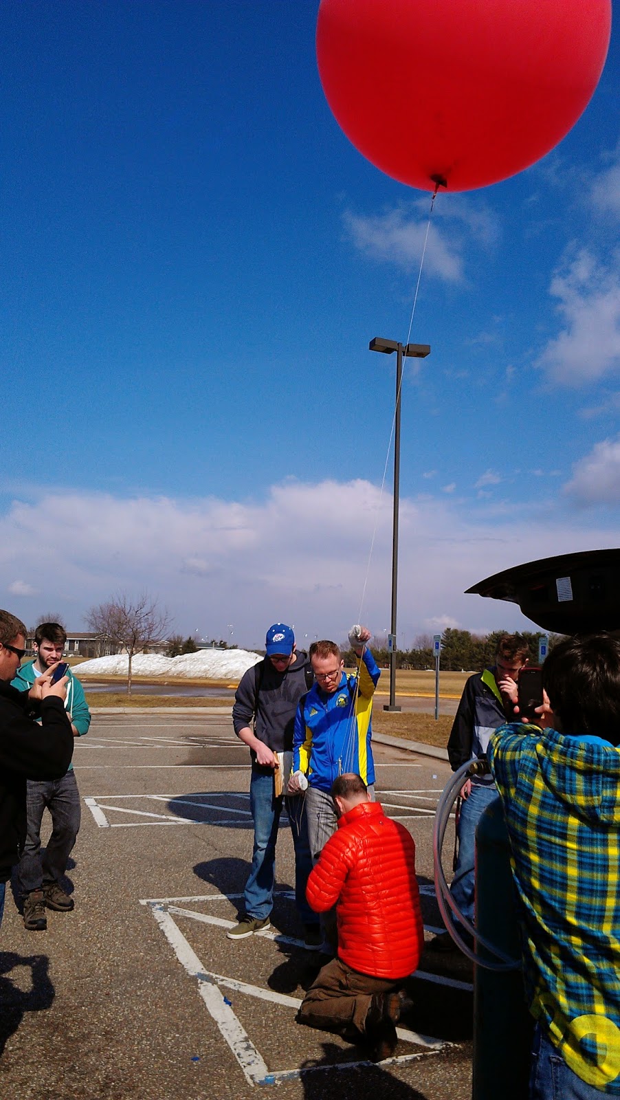
Figure 1. Dr. Hupy attaching the picavet rig to the line of the balloon. The rig contained a gps and two cameras, one with and one without geotagging capabilities.

 

The line was let out on the balloon until it reached about 500 feet. Since it was collecting images on the way up those images will be deleted before the mosaicking begins.

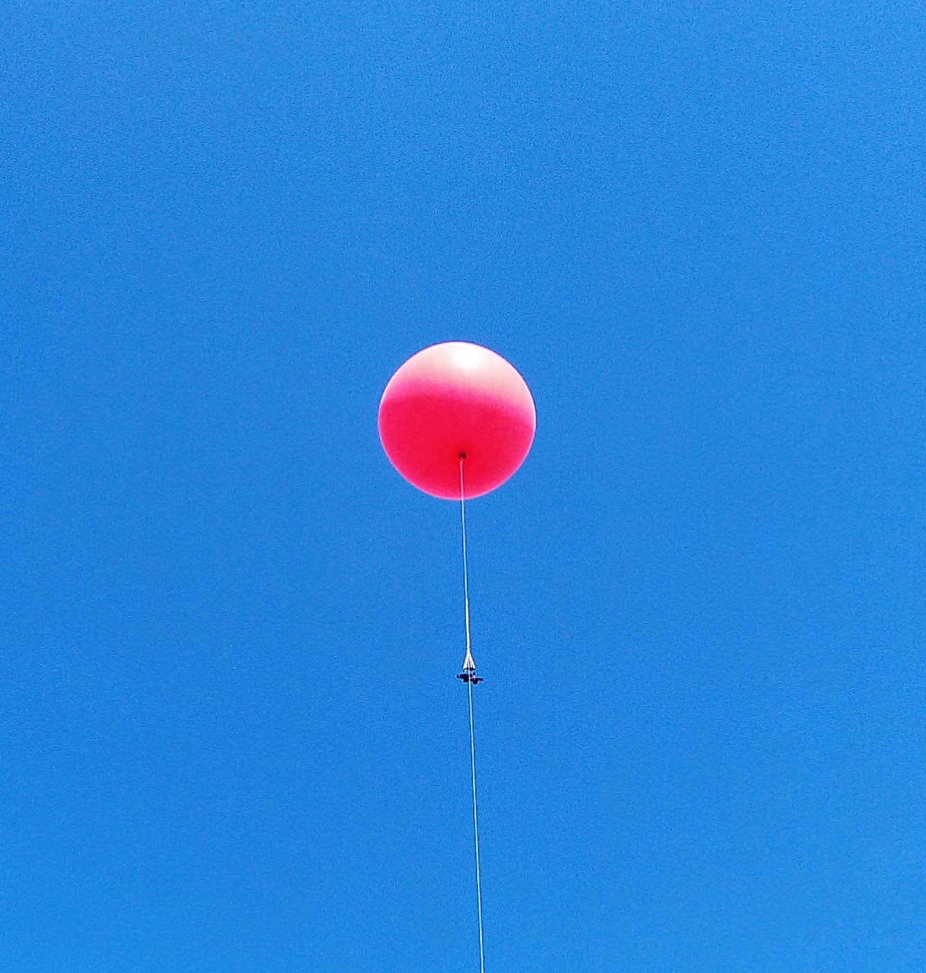
Figure 2. The balloon flying over us with both cameras collecting imagery.

 

We walked as a class around the fields making sure that the balloon was able to get imagery which would cover the entire study area. After roughly 45 minutes of walking we rendezvoused at the parking lot to reel in the balloon and begin to plan how to process the imagery.

In order to create the mosaicked image and DEM from the imagery we need to follow a set of directions to ensure that the images are processed correctly. The software used for the processing of the images was PhotoScan. Images used in PhotoScan do not need to be geotagged which is an advantage the software holds over other programs like Pix4D. If images were not geotagged that could be done by using GeoSetter which is an open source program that attaches coordinates to images and allows you to even embed a tracklog into a series of images. Embedding the tracklog into the images was very simple and fast but using PhotoScan, because of the computing power needed to analyze the pixels, can take several hours. Step by step directions for each program are below which track the process used for the final image and DEM.

PhotoScan Directions

1. On the Tab list click Workflow
2. Click Add Photos (only use the photos you want, if to many are used (~200) the process will take hours to complete)
3. Add the photos you want to stitch together
4. Once the photos are added go back to the Workflow tab and click Align Photos. This creates a Point Cloud, which is similar to LiDAR data.
5. After the photos are aligned in the Workflow tab, click Build Mesh. This creates a Triangular Integrated Network (TIN) from the Point Cloud.
6. After the TIN is created from the mesh, under Workflow click Create the Texture. Nothing will happen or appear different until you turn on the texture. 
7. Under the Tabs there will be a bunch of icons, some of them will be turned on all ready, but look for the one called Texture. Click on it to turn it on.
8. If you want you can turn off the blue squares by clicking on the Camera icon.
9. In order to export the image to use it in other programs; Under File, click Export Orthophoto.  You can save it as a JPEG/TIFF/PNG. It's best to save it as a TIFF.
10. With the photo exported as a TIFF, open ArcMap and bring in the TIFF photo and bring a satellite photo of Eau Claire or use the World Imagery base map.
11. You will only need to Georeference the photos if the images you are using were not Geotagged. Open the Geoprocessing Tool-set.
12. Click on the Viewer icon.  The button with the magnifying glass on.  This will open a separate viewer with the unreferenced TIFF in.
13. Click Add Control Points. The control points will help move the photo to where it is supposed to be.
14. With the control points click somewhere on the orthophoto, then click on the satellite image in ArcMap where the point in the unreferenced TIFF should be.  Keep adding control points until the photo is referenced.  The edges of the image will be distorted.  Don't spend too much time adding control points there.
15. The next step is to save the georeferenced image. Click on Georeferencing in the toolbar. Then click Rectify from the drop down menu.  You can save it wherever you need it.

Geosetter Directions

1.   First you will need to open the images that you will want to use. The photos will go into the viewer box on the left side of the screen. Look at all the photos and make sure there are not any blue markers on them. If they have black/grey they have lat/long attached to them.

2.   Click the icon circled and labeled 2 in figure 3.  This allows you to select the tracklog that you want to embed in the images.

3.   A window will open. Click Synchronize with Data File. Input the GPX track log (figure 3).

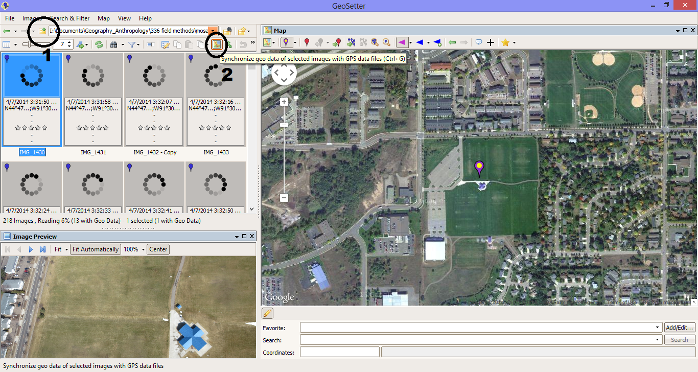
Figure 3. The GeoSetter interface.

 

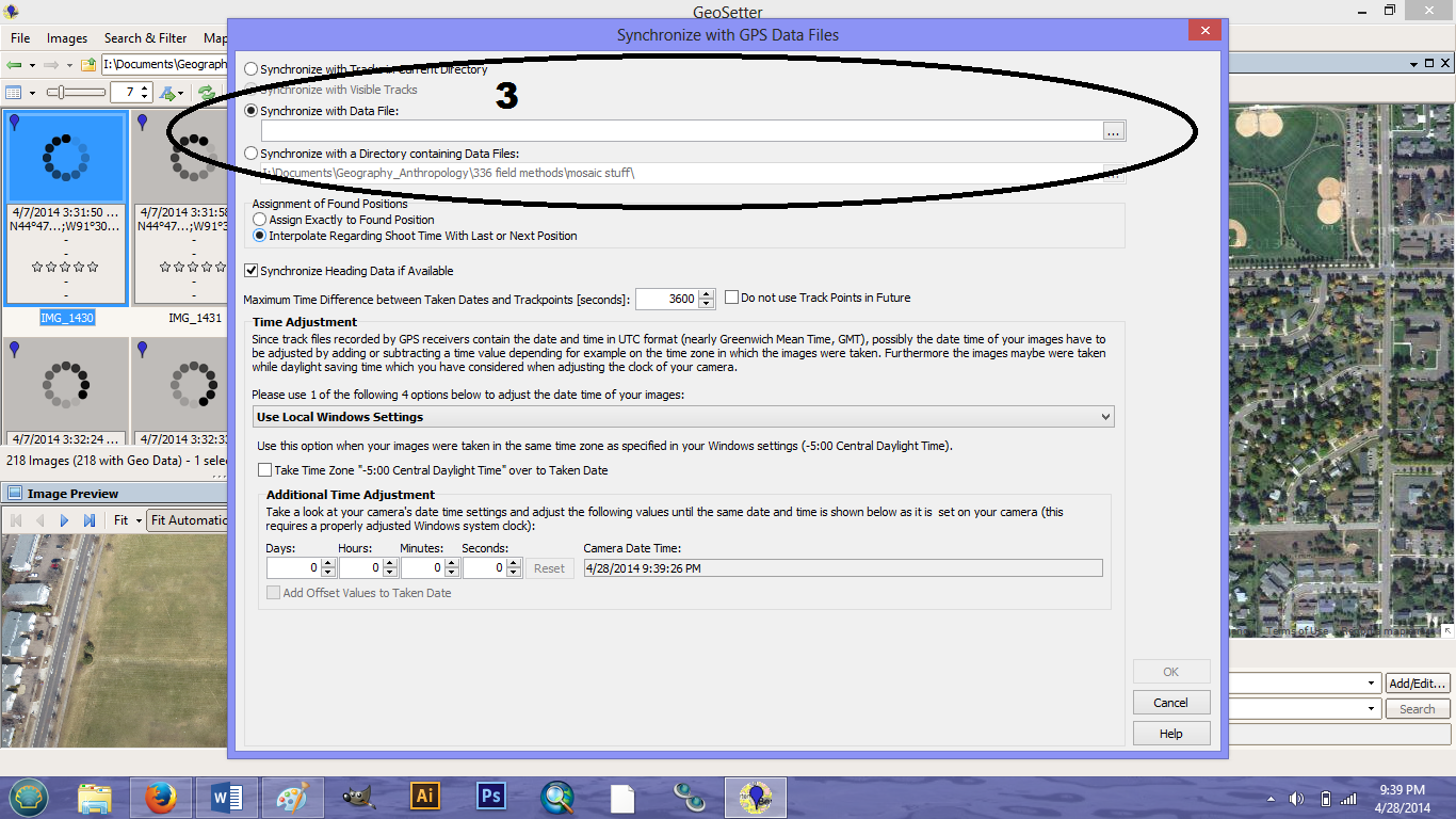
Figure 4. Embedding the tracklog by time into the images.

 

4.   To save the images simply close out of the program. A prompt will ask if you would like to save your changes. Click yes. This will save the coordinates on the images.

Results

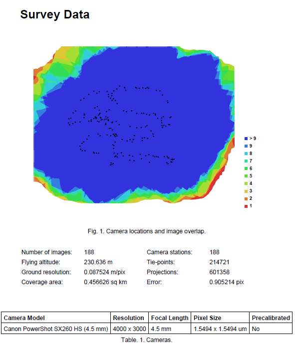
Figure 5. Image showing the amount of overlap of the images used in the mosaicking process.

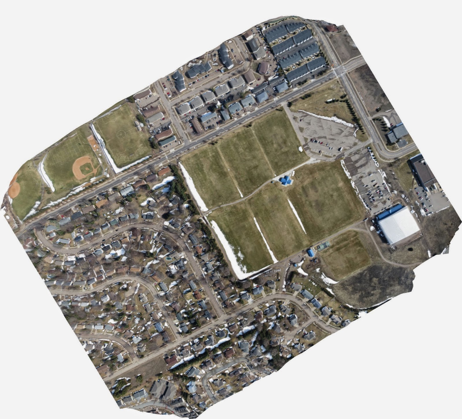
Figure 6. The resulting mosaic of the images which were not geotagged. The image is correct but the orientation is way off. This was corrected using Photoshop then georeferenced in ArcMap

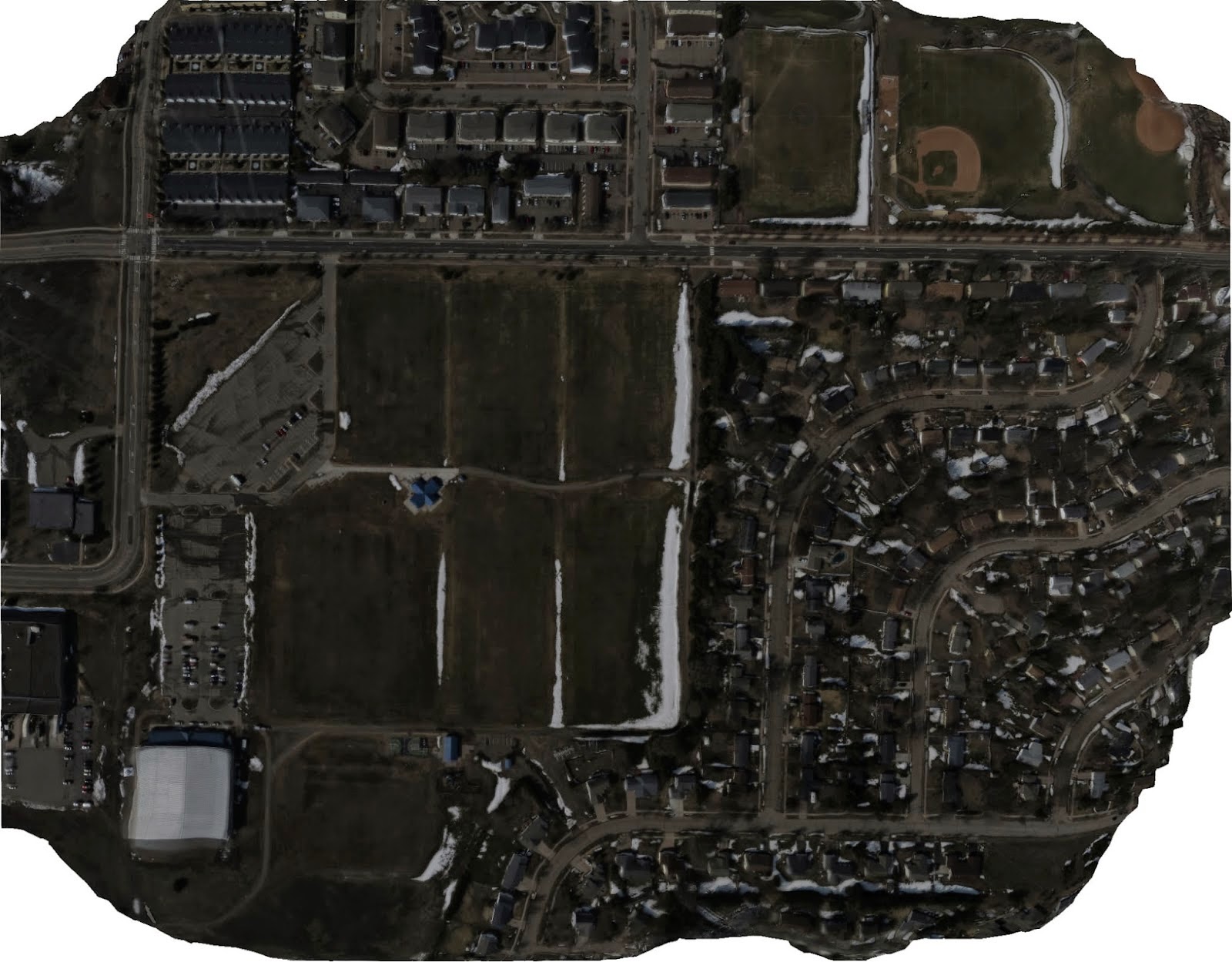
Figure 7. The resulting mosaic of the geotagged images from the other camera. Even those the image is a bit darker some minor adjustments to the contrast in photoshop can fix it quickly.

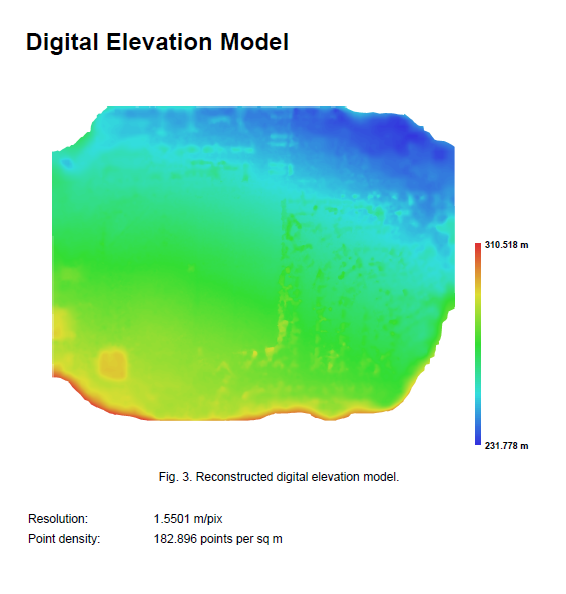
Figure 8. The DEM of the mosaicked geotagged images. This model is extremely accuate but upon close inspections many improvements could be made by collecting more imagery.

Discussion

It was found that using images that were not geotagged in PhotoScan caused the final image to be mirrored. This was easily fixed by rotating and flipping the tool inn photoshop but it could also be fixed by first embedding the tracklog into the untagged photos and then using them in PhotoScan. The final mosaics for the images look nearly seamless with no noticeable errors. The only areas of the mosaicked images with noticeable errors are the edges but this area could be clipped out leaving an image with almost no parallax (meaning that the final image would be what it would look like if the camera was shooting straight down).

Conclusions

The balloon with the picavet rig worked extremely well for this kind of project. A pricey UAV could have been employed which would have collected better images but with the balloon we were not limited to a flight time. PhotoScan and GeoSetter are two amazing programs for this kind of photogrammetry. Both were easy to use and the results were easy to work with and export into other programs such as ArcMap. A major pitfall of the balloon is that in bad weather (windy) it is ill-advised to collect any imagery with a balloon because it will be much harder to control than a kite or a remote controlled UAV would be.

Orienteering Exercise

This week’s class focused on using the compass skills we learned a few weeks ago in a real world setting. The location is the Priory on the south side of Eau Claire, WI just south of Interstate-94. The area is mostly wooded and is now the present site of a dormitory and the UWEC children’s center. There were maps made in an earlier blog which show the location and include a detailed account of the study area. 

Orienteering is defined as “a sport in which people use a map and a compass to travel along a route they do not know as quickly as possible” – MW dictionary. For this exercise we were given a compass, two maps with grids both in meters and degrees, and a list of checkpoints with coordinates in decimal degrees and meters. There were a few steps included in the orienteering exercise. 1, plot the coordinates on a map. 2, head to starting point and figure out azimuth and distance to first point. 3, send a “runner” ahead to a specified point. 4, a pace counter will count their steps as they head to where the runner is. This is to help estimate how much further the checkpoint is. 5, once the team arrives at a checkpoint repeat steps 1-4 for the next one.

 

Figure 1. Our pace counter on his way to where the runner was. Avoiding brush as the pace counter was difficult because it meant that his count may be inaccurate. The pace counter needed to be able to count only steps which reached the runner on a bee-line.

Figure 2. Calculating the distance traveled from the last point and the azimuth to the next point.

My group was given a list of five checkpoints to reach and an issue we ran into right away with plotting the points was that the grid for the map in degrees used seconds and minutes whereas the coordinates given were in decimal degrees so one of the group members spent extra time to convert the decimal degrees and compared his points to the points on the map in meters and found they were very similar. 

Figure 3. A map showing the location of the checkpoints with lines drawn to show the direction to each point.

Once the maps were filled with the checkpoints we started the exercise. From the starting point one member found the azimuth, my job as runner was to run ahead and help clear a path. Then the pace counter followed. The first point was easy to navigate to but we quickly learned that this exercise was not going to be fun.

Figure 4. The location of the second checkpoint was at the bottom of a ravine located under fallen brush and logs. Getting in and out of this ravine was a tremendous ordeal and not something fun.

The underbrush in the forested area was a lot thicker than I had anticipated. Luckily I wore jeans and appropriate shoes to keep my legs free of scrapes and scratches from all of the barbed bushes. Climbing out of the ravine from point two I started to slip so I reached to grab something, not looking, and grabbed a branch of something that was filled with barbs many of which broke off and stuck in my hand. A day after the exercise I found a barb still stuck in my thumb so I’m sure there are a few more barbs on me somewhere. 

We have been with the same group for almost every exercise this semester and building up our trust in one-another throughout the semester was vital to this exercise as it would have been easy to get frustrated in these conditions. The temperature wasn’t a factor as it was a nice 70 degree day but it felt worse as we began to get sweaty from walking about a mile over the rough terrain of the Priory.

Figure 5. A much smaller ravine than at point two. In the background you can see someone in a green shirt for reference of how large this ravine is. Even though this ravine was easier to cross than the last one it still helped to make the course more challenging as we were on our way to the third point.

The next time we do this exercise it would be beneficial to have a map with labeled contours instead of just contours. Since the points came with an elevation we could have estimated our height to see if we were closer or further from a point. A shirt with long sleeves and light gloves would help out with preventing cuts and scrapes. One of my friends decided to cut his jeans into shorts right before starting the course which turned out to be a major mistake for him as his legs we severely cut up by the end.